One thing that perhaps is lost when you first start working with ROOT, the need is to divide your ROOT analysis from your graph/histogram plotting. In your ROOT analysis you write the histograms/graphs to a file. Drawing the histograms, perhaps fitting, superimposing and using colours and different typess of line to differentiate should be performed by a much simpler macro. This way you can easily create/recreate figures that can be added to talks and reports without the need to rerun your analysis.
There are a number of examples shown in this page of common problems encountered. More examples can be found in the ROOT tutorial page and the HOW-TO ROOT page. The examples presented in this page, may or may not compile. Some of them are extracted from bigger macros to show a functionality of ROOT.
An example of a rootlogon.C macro is:
{// rootlogon.C
printf("\nWelcome to Sydney HEP rootlogon \n\n");     // print a message
gROOT->SetStyle("Plain");                       // plain histogram style
gStyle->SetOptStat("nemruoi");                  // expanded stats box
gStyle->SetPadTickX(1);                         // tic marks on all axes
gStyle->SetPadTickY(1);                         //
gStyle->SetOptFit(1111);                        // the results of the fits
gStyle->SetPadGridX(kTRUE);                     // draw horizontal and vertical grids
gStyle->SetPadGridY(kTRUE);
gStyle->SetPalette(1,0);                        // pretty and useful palette
gStyle->SetHistLineWidth(2);                    // a thicker histogram line
gStyle->SetFrameFillColor(10);                  // a different frame colour
gStyle->SetTitleFillColor(33);                 // title colour to highlight it
gStyle->SetTitleW(.77);                         // Title Width
gStyle->SetTitleH(.07);                        // Title height
gStyle->SetHistMinimumZero(true);               // Suppresses Histogram Zero Supression

}
If your analysis has more than 5 histograms then you may want to consider using the following to avoid having to define uniquely variable for all of them. We will use the ROOT has a container called TClonesArray to keep the same type of histogram. First lets define a class called HistDefTH1F that will contain all the information for 1D float histograms (TH1F). It easy enough to expand this for any type of histogram as shown in the code for TH2F (2D histograms) and TF1. This is actually used in a number of macros used by the ATLAS experiment.
#include <TH1F.h>
#include <TH2F.h>
#include <TProfile.h>
#include <TClonesArray.h>

class HistDefTH1F{
  public:
    Text_t *name;
    Text_t *title;
    Int_t nbins;
    Float_t xlow;
    Float_t xhigh;
};

class HistDefTH2F{
  public:
    Text_t *name;
    Text_t *title;
    Int_t n1bins;
    Float_t x1low;
    Float_t x1high;
    Int_t n2bins;
    Float_t x2low;
    Float_t x2high;
};

class HistDefTProf{
  public:
    Text_t *name;
    Text_t *title;
    Int_t nbins;
    Float_t x1low;
    Float_t x1high;
    Float_t x2low;
    Float_t x2high;
};
Lets create a global variable of type HistDefTH1F (and HistDefTH2F,HistDefTProf) where we initialise the parameters of the histograms that we need. In this example I defined a number of histograms: 1001, 1011, 1101. Remember to keep the numbers unique since this will be used to retrieve them from the container. Here we define histograms with 7 bins and limits between -0.5 and 6.5. This will ensure the bins are centered around the integer value.
HistDefTH1F histoTH1F[] = {
  { "hist1001",  "Ntracks Et>1GeV t1p3p"               , 7  ,  -0.5 ,    6.5 },
  { "hist1011",  "Passed Ntracks Et>1GeV t1p3p"        , 7  ,  -0.5 ,    6.5 },
  { "hist1101",  "Matched Ntracks Et>1GeV t1p3p"       , 7  ,  -0.5 ,    6.5 },
 { 0         , 0                                , 0  , 0.0 , 0.0}
};

HistDefTH2F histoTH2F[] = {

  {"hist2002","Number of Tracks Vs Energy"      , 5  , -0.5 , 4.5, 100  , 0.0 , 200.0},
  { 0   , 0                                   , 0  , 0.0 , 0.0, 0  , 0.0 , 0.0}
};

HistDefTProf histoTProf[] = {

  {"hist10101","   "                            ,20, 0.0, 100.0, 0.0, 100.0},
  {"hist10102","   "                            ,20, -3.0, 3.0, 0.0, 100.0},
  {"hist10103","   "                            ,20, -3.5, 3.5, 0.0, 100.0},
  {"hist10111","   "                            ,20, 0.0, 100.0, 0.0, 100.0},
  {0,0,0,0,0,0,0}
};
The last two snippets of code would be located within the header file. The next step is to define the TClonesArray member variable that will be part of the analysis class together with the functions that will be used by the analysis class to create, save and recall individual histograms. Remember to add #include <TClonesArray.h> near the top of the header.
   void CreateHistos();
   void StoreHistos(const char *name);
   TH1F       *GetHistoTH1F(Int_t x);  // returns Histogram with name "histX"
   TH2F       *GetHistoTH2F(Int_t x);  // returns Histogram with name "histX"
   TProfile   *GetHistoTProf(Int_t x);  // returns Histogram with name "histX"


private:
   TClonesArray      *m_histoTH1F;  // list of histograms TH1F
   TClonesArray      *m_histoTH2F;  // list of histograms TH2F
   TClonesArray      *m_histoTProf; // list of TProfiles
The last step is to define the three functions shown above:
void CollTree::CreateHistos()
{
  //  Create histograms... the bins, names are  held in histoTH1F

  Int_t i=0;
  m_histoTH1F = new TClonesArray("TH1F",5);
  TClonesArray &a=*m_histoTH1F;
  while (histoTH1F[i].nbins) {
    a[i]=new(a[i]) TH1F( histoTH1F[i].name,
        histoTH1F[i].title,
        histoTH1F[i].nbins,
        histoTH1F[i].xlow,
        histoTH1F[i].xhigh);
    i++;
  }

  m_histoTH2F = new TClonesArray("TH2F",8);
  TClonesArray &b=*m_histoTH2F;
  i=0;
  while (histoTH2F[i].n1bins) {
    b[i]=new(b[i]) TH2F( histoTH2F[i].name,
        histoTH2F[i].title,
        histoTH2F[i].n1bins,
        histoTH2F[i].x1low,
        histoTH2F[i].x1high,
        histoTH2F[i].n2bins,
        histoTH2F[i].x2low,
        histoTH2F[i].x2high);
    i++;
  };
  m_histoTProf = new TClonesArray("TProfile",7);
  TClonesArray &c=*m_histoTProf;
  i=0;
  while (histoTProf[i].nbins) {
    c[i]=new(c[i]) TProfile( histoTProf[i].name,
        histoTProf[i].title,
        histoTProf[i].nbins,
        histoTProf[i].x1low,
        histoTProf[i].x1high,
        histoTProf[i].x2low,
        histoTProf[i].x2high);
    //			     histoTProf->at(i).x2high,
    //			     "s");
    i++;
  };

};
//_________________________________________________________________________
void CollTree::StoreHistos(const char *name)
{ // writes all the histograms individually defined in m_histoTH1F in the same root file
  TFile f(name,"RECREATE");

  //store histograms

  m_histoTH1F->Write();
  m_histoTH2F->Write();
  m_histoTProf->Write();
}

//_________________________________________________________________________
TH1F *CollTree::GetHistoTH1F(Int_t x)
{// returns the histogram specified by the number
  Text_t name[500];
  sprintf(name,"hist%04d",x);
  return (TH1F*) m_histoTH1F->FindObject(name);
}

//_________________________________________________________________________
TH2F *CollTree::GetHistoTH2F(Int_t x)
  //_________________________________________________________________________
{
  Text_t name[20];
  sprintf(name,"hist%04d",x);
  return (TH2F*) m_histoTH2F->FindObject(name);
}
//_________________________________________________________________________
TProfile *CollTree::GetHistoTProf(Int_t x)
  //_________________________________________________________________________
{
  Text_t name[20];
  sprintf(name,"hist%04d",x);
  return (TProfile*) m_histoTProf->FindObject(name);
}
The functions CreateHistos() and StoreHistos() should all be called once. Before any histogram work is to be done and after all the histogram work is done respectively. GetHistoTH1F() should be called whenever you need to get the pointer to the desired histogram. For example if you want to get a distribution of a parameter that changes with respect to event, the following line would be placed inside the loop to fill histogram 1001 with the correct variable.
GetHistoTH1F(1001)->Fill((float)N_Tracks);
The advantage of this method is that it provides you with a simple way to manage your histograms. To add new histograms you only have to add elements to the HistDefTH1F array or any of the other relevant arrays.
To save a histogram into a eps(useful for latex), pdf or a number of formats available in ROOT, the command Print that is a method of TCanvas has to be invoked. Here an example that show how this is done as well as other histogram manipulations that are useful when polishing histograms for reports and talks.(Not all the variables are defined!!)
 TCanvas *c = new TCanvas("c1","canvas",800,600);
 c->SetFillColor(10); // the white background
 c->SetFillColor(10); // hopefully you set your rootlogon.C so you do not have to do this
 gPad->SetFillColor(10);
 c->SetGridx(); // set the grid
 c->SetGridy();

 histo->SetTitle("MSSM Higgs Visible Mass");
 histo->GetXaxis()->SetTitle("Mass(GeV)");
 histo->GetYaxis()->SetTitleOffset(1.2); // too close to the axis lets move it a bit
 histo->SetLineColor(8);
 histo->SetFillColor(8);

// lets create the filenames to save the graphs
 sprintf(eps_filename,"%s.eps",filename_eps);
 sprintf(image_filename,"%s.jpg",filename_jpg);

 // lets save the graphs
 c->Print(eps_filename);
 c->Print(image_filename);
Making a copy of the histogram as an image is useful for viewing and perhaps for just copying into a presentation. In the HEP PC KuickShow (located under the graphics menu) can be used to view the images. By pressing page up or page down it will display the next or the previous image in the directory.
A method to extract TObjects that have been saved to a file is shown. You can either type each command at prompt or execute the macro. In this example we will return the TGraph( A kind of TOBject) "DalitzPlot" that has been saved in the root file(filename).
TGraph*
Get_TGraph(char *filename)
{

 TFile *theFile = new TFile(filename);
 // to list all the directories and TObjects in the file, TTrees, TGraphs, TH1.. etc
  theFile->ls();

// Get by default returns a TObject, hence we need to typecast it
 TGraph *theGraph = (TGraph*)theFile->Get("DalitzPlot");

 if (theGraph != NULL) // check we got something useful
   theGraph->Draw("ALP"); // lets draw it

 return theGraph;
}
When preparing many histograms it can be useful to have them all in one file. To place them on multiple pages in the one document the easiest way is to add parenthesis as shown in the example below. (Another way is to call the TImage class:
TCanvas c1("c1"); // assumes that histograms h1,h2 and h3 are defined elsewhere
h1.Draw();
c1.Print("c1.ps(");  // write canvas and keep the ps file open
h2.Draw();
c1.Print("c1.ps");   // canvas is added to "c1.ps"
h3.Draw();
c1.Print("c1.ps)");  // canvas is added to "c1.ps" and ps file is closed
Afterwards you can run "ps2pdf c1.ps output.pdf" to convert the file to the pdf format.
There are several ways of doing this. Here is one way, using the TObjArray class. Whilst not necessarily the best way, it does work. This example defines three TLorentzVector objects, and makes a list of pointers to them. The list is then looped through. To try this, save the code to a file named tobjarray_example.cc and at the root prompt, type
.x tobjarray_example.cc
Here is the code:
{
   // File: tobjarray_example.cc
   //
   // Using TObjArray class
   // ~~~~~~~~~~~~~~~~~~~~~
   //
   // This approach should work with any root object which derives from the
   // TObject class. Here we use TLorentzVector objects
   //
   // To use, run root and at the prompt type
   //               .x tobjarray_example.cc
   //
   // Declaration:

#include <TObjArray.h>

   TObjArray* object_list = new TObjArray();

   // Adding something to the list:

   TLorentzVector v1(0., 0., 0., .1395);
   TLorentzVector v2(0., 0., 0., .938);
   TLorentzVector v3(0., 0., 0., 1.777);

   TLorentzVector* p1 = &v1;
   TLorentzVector* p2 = &v2;
   TLorentzVector* p3 = &v3;

   object_list->AddLast(p1);
   object_list->AddLast(p2);
   object_list->AddLast(p3);

   // Looping through list. (Note we cast the object to the type we need)

   TObjArrayIter next(object_list);
   TObject* object;
   while ( ( object = next() ) ) {
        // Do something with object
        TLorentzVector* p = (TLorentzVector*) object;
        std::cout << "Mass is: " << p->M() << std::endl;
   }

}
The axes of your graphs and histograms should always have titles. It is a good idea to get into the habit to set them the first time you draw them. This will help you avoid the common missing titles and units on graphs/histograms when reports, papers are printed for proof reading. In ROOT this can be easily achieved. A simple examples for a histogram is:
void Plot_Histo()
{// this function will plot a 1D histogram

 // TH1F *histo = new TH1F("RecElecRatio","RecElecRatio",100,0,120);

  TFile *file = new TFile("filename.root");

   TH1F *histo = file->Get("HistogramName");

  // do whatever filling you would like to do

  // lets set the axes
  // you can set all three axes with one command
  // the value of the histogram title, x and y are separated by ;
  // Remember you can use latex to do your symbols
  histo->SetTitle("Transverse Momentum ratio for electrons;Pt_{Rec}/Pt_{Truth};Number");
  histo->Draw("");
}
All the latex functions available in ROOT are listed in this chapter of the ROOT manual.
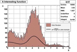
The output of Draw_Legends() To provide a useful description of the graphs or histograms being presented in the same plot is very easy with the TLegend object. In this example a formula and a histogram are plotted together with a legend explaining what they are.
void Draw_Legends()
{
   TCanvas *c1 = new TCanvas("c1","The Legend Example");
   c1->SetFillColor(0);

   TLegend *legend = new TLegend(0.4,0.6,0.89,0.89);

   TFormula *form1 = new TFormula("form1","abs(sin(x)/x)");
   TF1 *sqroot = new TF1("sqroot","x*gaus(0) + [3]*form1",0,10);
   sqroot->SetParameters(10,4,1,20);

   TH1F *histo = new TH1F("h1f","Test random numbers",200,0,10);
   histo->SetFillColor(45);
   histo->FillRandom("sqroot",10000);

   histo->Draw();
   sqroot->Draw("same"); // so it superimposes the function on the histogram

   // now lets add the different features of the graph that we want to explain
   // the syntax is feature or object (Histo, graph, formular etc), description,
   // what we want to show
   // this could be the marker "p", the fill colour "f" or the line colour "l"
   legend->AddEntry(histo,"Histo Random", "f");
   legend->AddEntry(sqroot,"xe^{x^{2}}|#frac{sin(x)}{x}| a Latex example", "l");

   legend->Draw(); // it will draw it in the position that was created..
                   // but it can be moved with the mouse
   c1->Update();
}
Most people know that to superimpose histograms you can use Draw("SAME") but you only get one statbox drawn. To draw all of them you need to use "SAMES" . The statbox is only available once the histogram is drawn to access, in case you want to change the colours of the font or its position, look at the following code:
void Draw_StatBoxExample()
{
  char name[30];
  float Nsig = 20.4; // nothing too serious
  TCanvas *c1 = new TCanvas("c1","The Legend Example");
  c1->SetFillColor(0);

  // to generate the graph
  TFormula *form1 = new TFormula("form1","abs(sin(x)/x)");
  TF1 *sqroot = new TF1("sqroot","x*gaus(0) + [3]*form1",0,10);
  sqroot->SetParameters(10,4,1,20);


  TH1F *histo = new TH1F("h1f","Test random numbers",200,0,10);
  histo->SetFillColor(45);
  histo->FillRandom("sqroot",100);
  histo->Draw("");

  c1->Update();
//  TPaveStats *st = (TPaveStats*)histo->GetListOfFunctions()->FindObject("stats"); get it from the histogram
  TPaveStats *st = (TPaveStats*)c1->GetPrimitive("stats");
  if (st != NULL) {
    st->SetY1NDC(.4);  // bottom
    st->SetY2NDC(.6);  // top
    st->SetX1NDC(.8);  // left
    st->SetX2NDC(1);  // right
    st->SetTextColor(2);  // the colour of the font being used by the pavestat

    // if you want to add text you will need to clone it
    sprintf(name, "MyVal = %.0f", Nsig);
    TString text_line = TString(name);
    st->AddText(text_line.Data());
    st->DrawClone();

  //    st->Print();  // you can call Print to see if the text you set it is correct

  }

  c1->Modified(); //important otherwise you will not see your changes
  c1->Update();
}
In the following link you will find definition of constants to specify colour, style and types for text,line,fills and markers.
Here is an example that shows how to read an ascii file into a number of histograms.
ReadTextFile()
{
   gROOT->Reset();

   TCanvas *c1 = new TCanvas("c1","Axial Sensitivity",200,10,600,400);
   //TCanvas *c2 = new TCanvas("c2","Two Graphs",200,10,600,400);

   TH1F *AS18 = new TH1F("AS18","Axial sensitivity",50,-100.,+100.);
   TH1F *AS20 = new TH1F("AS20","Axial sensitivity",50,-100.,+100.);
   TH1F *AS22 = new TH1F("AS22","Axial sensitivity",50,-100.,+100.);

   Float_t         z;

   FILE *out;
// each input file is one column but you can easily see how you could modify
// fscanf to include more columns
   out=fopen("18.txt","r"); while(!feof(out)){ fscanf(out,"%f",&z); AS18->Fill(z);}
   fclose(out);
   out=fopen("20.txt","r"); while(!feof(out)){ fscanf(out,"%f",&z); AS20->Fill(z);}
   fclose(out);
   out=fopen("22.txt","r"); while(!feof(out)){ fscanf(out,"%f",&z); AS22->Fill(z);}
   fclose(out);

   AS22->GetXaxis()->SetTitle("Axial position (mm)");
   AS22->GetYaxis()->SetTitle("Counts");

   AS22->SetFillColor(1);AS22->SetMarkerStyle(23); AS22->SetMarkerColor(1);
   AS22->Draw();
   AS20->SetFillColor(2);AS20->SetMarkerStyle(22); AS20->SetMarkerColor(2);
   AS20->Draw("same");
   AS18->SetFillColor(3);AS18->SetMarkerStyle(21); AS18->SetMarkerColor(3);
   AS18->Draw("same");

   AS22->SetStats(0); // no statbox on the canvas
   TLegend *legend = new TLegend(.75,.80,.95,.95);
   legend->AddEntry(AS18,"18 mm");
   legend->AddEntry(AS20,"20 mm");
   legend->AddEntry(AS22,"22 mm");
   legend->Draw("");
}
Lets say you have your own macro with its function that you compile within ROOT. Everybody knows about .L command and adding the + sign at the end of the file to invoke the ROOT compiler. What if you wanted to do this within a macro so you do not have to type command all the time. In the following macro the ROOT class TSystem is introduced to achieve this. The example also shows how to load shared libraries and add include paths so that the compilation finds the correct header files.
In the example, the shared libraries, TauPerformNtuple and TrigTauPerformAnalysis are loaded (the ROOT Physics is also explicitly loaded since it is required by the former shared libraries). The function mcTruthPlots is implemented in mcTruthPlots.cxx which is compiled on the go if any changes have occurred since the last time it was compiled otherwise just load the shared library mcTruthPlots_cxx.so that was created previously. The macro LetsStart.C is:
void LetsStart()
{// we use this function to run everything

// lets load the physics library, otherwise the next two libraries will not
// find things such as TLorentzVector
gSystem->Load("libPhysics");
// our functions
gSystem->Load("libTrigTauPerformNtuple.so");
gSystem->Load("libTrigTauPerformAnalysis.so");

// additional include path to find the header files specified in mcTruthPlots.cxx
// note the need to use the flag -I
gSystem->AddIncludePath("-ITrigTauAnalysis/TrigTauPerformAnalysis");
gSystem->AddIncludePath("-ITrigTauAnalysis/TrigTauPerformNtuple");

// lets see the include path that was defined
// for debugging
printf("Include path %s\n",gSystem->GetIncludePath());

// the macro that will be using
// this will compile the macro and loaded if the compilation is successful
gSystem->CompileMacro("mcTruthPlots.cxx","k");

// run the function defined in the macro [Note "xx" "yy" concat]
mcTruthPlots("trig1_misal1_mc12.005188.A3_Ztautau_filter.recon"
		".AOD.v13003003_tid017923.TTP06.merged.0.root");

}
The ROOT commands to execute the macro would be:
.L LetsStart.C
LetsStart()
In this example, the code shown below shows how to read a number of root files that contain the same TTree structure but with different data. Here the TTree class is called CollectionTree .
void ReadTree()
{// all the root files are listed in the Ztautau_tid007904_list_Ntuple.txt

  TChain *chain = new TChain("CollectionTree");

  FILE *input;
  char filename[300];

  input = fopen("Ztautau_tid9169_list_Ntuple.txt","r");
  if (input != NULL) { // lets read each line and get the filename from it
    while (fscanf(input,"%s\n",filename) != EOF) {
      printf("%s\n",filename);
      chain->Add(filename);
    }

   fclose(input);
// the TTree class created with makeclass is called RecoTau
// and it has a method with which to intitialise the TTree
   RecoTau  CompleteTree(chain);

// do the analysis with the methods defined in RecoTau
   CompleteTree.CreateHistos();
   CompleteTree.Loop();
   CompleteTree.StoreHistos("histos_tauRec_test2_vis.root");


}
Sometimes the Aclic compiler that comes with ROOT takes its time compiling, especially if you are using vectors. One way to avoid this
is to use another compiler, include the ROOT libraries so you can do histogramming and employ the rest of the ROOT capabilities. To be able to do this, you have to make sure your C++ code is not sloppy. Everything is defined and all the required include files are listed. To get all the libraries required link and directories for the version of ROOT you are using, ROOT has a utility called 'root-config' which returns a string with information specified.
Here is an example where we compile a fictitious program called Tau_Rec.cpp .This program reads a root file with a TTree and creates a file with a number of histograms. So we need to specify the ROOT include directory plus the libraries required by the linker.
flags=$(root-config --incdir --libs)
g++ Tau_Rec.cpp -o TauRec  -I$flags
Now $flags corresponds to $ROOTSYS/include -L$ROOTSYS/lib -lCore -lCint -lRIO -lNet -lHist -lGraf -lGraf3d -lGpad -lTree -lRint -lPostscript -lMatrix -lPhysics -lMathCore -lThread -pthread -lm -ldl -rdynamic
You depending on your code you may need the standard library -lstdc++ to be included as well.
The library -ldl is necessary otherwise you will get errors such as:
/usr/physics/hep/root/lib/libCint.so: undefined reference to `dlerror'
/usr/physics/hep/root/lib/libCore.so: undefined reference to `dladdr'
/usr/physics/hep/root/lib/libCint.so: undefined reference to `dlclose'
/usr/physics/hep/root/lib/libCint.so: undefined reference to `dlopen'
/usr/physics/hep/root/lib/libCint.so: undefined reference to `dlsym'

The output of Draw_Normalised()
This macro shows how to superimpose two histograms that have been read from two different files. The superimposition is performed using the THStack object. The stat boxes are moved and resize to fit outside the actual histogram together with the legend. This function gets the histograms from a root file. If the histograms are already in memory you will need to modify the code slightly.
The macro as it is, draw the two histograms as normalised.
void
Draw_Normalised(char *histoname1, char *histoname2, bool normalised)
{// this function draws the histoname from both files superimposed
 // and normalised
  TObjArray RootFiles;
  TObjArray histos;

  int i;
  // the colours to be used to differentiate the two histograms
  // stats and legends
  std::vector<int> colours;
  colours.push_back(1);
  colours.push_back(4);

  // the legend strings
  std::vector<std::string> legends_str;
  legends_str.push_back("Reference Plot");
  legends_str.push_back("New Plot");


  TFile *f_Ref = new TFile("Reference_Plots.root");
  if (!f_Ref->IsOpen()) {printf("Error opening Reference root file\n"); return 0;}

  TFile *f_New = new TFile("New_Plots.root");
  if (!f_New->IsOpen()) {printf("Error opening New root file\n"); return 0;}

  // lets add the first histogram
  TH1F* histo1 = f_Ref->Get(histoname1);
  if (histo1 != NULL)
  histos.AddLast(histo1);
  else {
      printf("Error getting histogram %s\n",histoname1);
      return 1;
  }

  // lets add the second histogram
  TH1F* histo2 = f_New->Get(histoname2);
  if (histo2 != NULL)
  histos.AddLast(histo2);
  else {
      printf("Error getting histogram %s\n",histoname2);
      return 1;
  }


 // lets open and draw the canvas
  TCanvas *canvas = new TCanvas("c5","TauValidation");
  canvas->SetTicks(0,0);
  canvas->SetRightMargin(0.20);

  // lets take the first histoname and see if we can match a title to
  // its which will be HS stack title

  THStack *Hs = new THStack("hs2","Stack Title");

// we need different positions for the legend to not
  TLegend  *legend = new TLegend(0.80,0.3,0.995,0.4);

  for (i=0;i<histos.GetEntries();i++)
  {
    TH1F *h =  (TH1F*)histos[i];

    if (normalised) {
      double val1 = h->GetSumOfWeights();
      if (fabs(val1) > 0)
        h->Scale(1.0/val1);
    }

    h->SetLineWidth(2);
    h->SetLineColor(colours[i]);


    if (i== 0) {// the reference
      h->SetFillColor(17); // light gray
      h->SetFillStyle(3001);
    }


    legend->AddEntry(h,legends_str[i].c_str(),"L");
    Hs->Add(h,"sames");

  }

  float heightboxes;
  // the position of the top corner
  float top_corner,deltay;
  // don't draw errors if it is 1
  int no_error = 0;
  top_corner = 0.9;

  // if the array has more than 0 histograms lets specify the stat boxes and determine
  // whether we should draw errors
  if (histos.GetEntries() > 0) {

    heightboxes = (float)0.5/(float)histos.GetEntries();
    if ((strcmp(histos.At(0)->GetName(),"hist7132") == 0)
     || (strcmp(histos.At(0)->GetName(),"hist7032")))
      no_error = 1;
  }
  else
    heightboxes = (float)0.5;


  TPaveStats *st1;

  if (no_error == 1) // do not draw errors
    Hs->Draw("HIST nostack");
  else
    Hs->Draw("HISTE nostack");

  canvas->Update();

  for (i=0;i<histos.GetEntries();i++)
  {
    TH1F *h =  (TH1F*)histos.At(i);
    if (h != NULL) {
      // lets modify the stat boxes
      deltay = i*heightboxes;
      st1 = (TPaveStats*)h->GetListOfFunctions()->FindObject("stats");
      if (st1 != NULL) {
        st1->SetOptStat(1111);
        st1->SetOptFit(0011);
        st1->SetStatFormat("2.3e");
        st1->SetFitFormat("2.3e");
        if (i == 0) {
          st1->SetFillColor(17); // light gray
          st1->SetFillStyle(3001);
        }
        else {
          st1->SetFillColor(0); //white
          st1->SetFillStyle(1001); //white
        }
        st1->SetY1NDC(top_corner-deltay-heightboxes); st1->SetY2NDC(top_corner-deltay);
        st1->SetX1NDC(0.80); st1->SetX2NDC(.995);
        st1->SetTextColor(colours[i]);
      }
      else
        printf("NULL\n");
    }
  }

  legend->Draw("");

  canvas->Update();
  canvas->Modified(); // so it updates the canvas with the new changes
  canvas->Draw("");

}
The output of Draw_Normalised() This version of the macro takes a TObjArray of histograms and plots them using the standard root colours starting at 1 = Black. Optional arguments are:
TPad *pad: the TPad where you want the histograms to be drawn. bool normalised: will normalise the histograms, default is false. std::string stacktitle: the title to be used for the plot, default will take the title of the first histogram.
In the example below, the plots are drawn on the 2nd TPad of the TCanvas.
TCanvas *cl = new TCanvas("cl","cl",1200,1000);
cl->Divide(2,2);
Draw_Normalised(histos, (TPad*)cl->cd(2));


void Draw_Normalised(TObjArray histos,
		TPad *pad = 0,
		bool normalised = false,
		std::string stacktitle = "")
{// this function draws the histoname from the TObjArray superimposed
 // and normalised if required

   if( histos.GetEntries() == 0 ) return;

  TObjArray RootFiles;
  std::vector<std::string> legends_str;
  std::vector<int> colours;


  for(int i = 0; i < histos.GetEntries(); i++){

     TH1F *h =  (TH1F*)histos[i];
     legends_str.push_back( h->GetTitle() );
     colours.push_back( i+1 );
  }


 // lets open and draw the canvas
  TCanvas *canvas;
  if(pad == 0){
     *canvas = new TCanvas("c5","TauValidation");
     pad = (TPad*)canvas->cd();
  }
  pad->cd();
  pad->SetTicks(0,0);
  pad->SetRightMargin(0.20);

  // lets take the first histoname and see if we can match a title to its which will be HS stack title

  if( stacktitle == "" ) stacktitle = ((TH1F*)histos[0])->GetTitle();
  THStack *Hs = new THStack("hs2",stacktitle.c_str());

  TLegend  *legend = new TLegend(0.80,0.3,0.995,0.4); // we need different positions for the legend to not

  for (i=0;i<histos.GetEntries();i++)
  {
    TH1F *h =  (TH1F*)histos[i];

    if (normalised) {
      double val1 = h->GetSumOfWeights();
      if (fabs(val1) > 0)
        h->Scale(1.0/val1);
    }

    h->SetLineWidth(2);
    h->SetLineColor(colours[i]);

    legend->AddEntry(h,legends_str[i].c_str(),"L");
    Hs->Add(h,"sames");

  }

  float heightboxes;
  // the position of the top corner
  float top_corner,deltay;
  // don't draw errors if it is 1
  int no_error = 0;
  top_corner = 0.9;

  // if the array has more than 0 histograms lets specify the stat boxes and determine whether we should
  // draw errors
  if (histos.GetEntries() > 0) {

    heightboxes = (float)0.5/(float)histos.GetEntries();
    if ((strcmp(histos.At(0)->GetName(),"hist7132") == 0) || (strcmp(histos.At(0)->GetName(),"hist7032")))
      no_error = 1;
  }
  else
    heightboxes = (float)0.5;


  TPaveStats *st1;

  if (no_error == 1) // do not draw errors
    Hs->Draw("HIST nostack");
  else
    Hs->Draw("HISTE nostack");

  pad->Update();

  for (i=0;i<histos.GetEntries();i++)
  {
    TH1F *h =  (TH1F*)histos.At(i);
    if (h != NULL) {
      // lets modify the stat boxes
      deltay = i*heightboxes;
      st1 = (TPaveStats*)h->GetListOfFunctions()->FindObject("stats");
      if (st1 != NULL) {
	 //st1->SetOptStat(1111);
        st1->SetOptFit(0011);
        st1->SetStatFormat("2.3e");
        st1->SetFitFormat("2.3e");
	st1->SetFillColor(19);

        st1->SetY1NDC(top_corner-deltay-heightboxes); st1->SetY2NDC(top_corner-deltay);
        st1->SetX1NDC(0.80); st1->SetX2NDC(.995);
        st1->SetTextColor(colours[i]);
      }
      else
        printf("NULL\n");
    }
  }

  legend->Draw("");

  pad->Update();
  pad->Modified(); // so it updates the pad with the new changes
  pad->Draw("");

  return;
}
When a stack is drawn without nostack each previous histogram is added to the next for the final display. In order to get the stats for the original histogram they must first be plotted with the nostack option, and then the stats boxes must be copied and drawn again after the stack is drawn.
void Draw_Stacked(TObjArray histos,
		     TPad *pad = 0,
		     bool normalised = false,
		     std::string stacktitle = "" )
{// this function draws histograms stacked and correctly takes into account the
 // stats boxes for each

   if( histos.GetEntries() == 0 ) return; // nothing to do

   // Initial set up
   TObjArray statsboxes;
   std::vector<std::string> legends_str;
   std::vector<int> colours;
   TPaveStats *st1;

   const int n = histos.GetEntries();

   // choose the colours
   for(int i = 0; i < histos.GetEntries(); i++){
      if(i+1<5) // I skip yellow
	 colours.push_back( i+1 );
      else
	 colours.push_back( i+2 );
   }


   // lets open and draw the canvas
   TCanvas *canvas;
   if(pad == 0){
      *canvas = new TCanvas("c5","Stacked Histograms");
      pad = (TPad*)canvas->cd();
   }
   pad->cd();
   pad->SetTicks(0,0);
   pad->SetRightMargin(0.20);

   // lets take the first histoname and see if we can match a title to its which will be HS stack title
   if( stacktitle == "" ) stacktitle = ((TH1F*)histos[0])->GetTitle();
   THStack *Hs = new THStack("hs2",stacktitle.c_str());

   // Set Axis Units
   //  Hs->GetXaxis()->SetTitle( ((TH1F*)histos[0])->GetXaxis()->GetTitle() );

   // Set up the LEGEND
   TLegend  *legend = new TLegend(0.80,0.3,0.995,0.4); // we need different positions for the legend to not
      // get the plot titles for the legend
   for(int i = n; i > 0 ; i--){

      TH1F *h =  (TH1F*)histos[i-1];
      legends_str.push_back( h->GetTitle() );
   }
   for (i=n-1;i>-1;i--) {
      TH1F *h =  (TH1F*)histos[i];
      legend->AddEntry(h,legends_str[n-1-i].c_str(),"L");
   }


   // Add and draw the plots
   for (i=0;i<histos.GetEntries();i++){
      TH1F *h =  (TH1F*)histos[i];

      if (normalised) {
	 double val1 = h->GetSumOfWeights();
	 if (fabs(val1) > 0)
	    h->Scale(1.0/val1);
      }

      h->SetLineWidth(0);
      h->SetLineColor(colours[n-1-i]);
      h->SetFillColor(colours[n-1-i]);

      Hs->Add(h,"sames");
   }

  float heightboxes;
  // the position of the top corner
  float top_corner,deltay;
  // don't draw errors if it is 1
  int no_error = 1;
  top_corner = 0.9;

  // if the array has more than 0 histograms lets specify the stat boxes
  if (histos.GetEntries() > 0) {
     heightboxes = (float)0.5/(float)histos.GetEntries();
  }
  else
     heightboxes = (float)0.5;

  // DRAW not stacked to get correct stats boxes
  if (no_error == 1) // do not draw errors
    Hs->Draw("HIST nostack");
  else
    Hs->Draw("HISTE nostack");

  pad->Update();

  // Work with stats boxes and save copy for later use
  for (i=histos.GetEntries()-1;i>-1;i--){
     TH1F *h =  (TH1F*)histos.At(n-i-1);
     if(h != NULL){

	// lets modify the stat boxes
	deltay = i*heightboxes;
	st1 = (TPaveStats*)h->GetListOfFunctions()->FindObject("stats");

	if (st1 != NULL) {
	   //st1->SetOptStat(1111);
	   st1->SetOptFit(0011);
	   st1->SetStatFormat("2.3e");
	   st1->SetFitFormat("2.3e");
	   st1->SetFillColor(19);

	   st1->SetY1NDC(top_corner-deltay-heightboxes); st1->SetY2NDC(top_corner-deltay);
	   st1->SetX1NDC(0.80); st1->SetX2NDC(.995);
	   st1->SetTextColor(colours[i]);

	   // Copy them for later
	   TPaveStats* temp = (TPaveStats*)st1->Clone();
	   statsboxes.AddLast(temp);
	}
	else{
	   printf("NULL\n");
	}
     }
  }

  pad->Update();
  pad->Modified(); // so it updates the pad with the new changes
  pad->Draw("");


  // DRAW finally stacked
  if (no_error == 1) // do not draw errors
     Hs->Draw("HIST");
  else
     Hs->Draw("HISTE");

  // Redraw correct stats boxes
  for (i=histos.GetEntries()-1;i>-1;i--){
     ((TPaveStats*)statsboxes.At(n-i-1))->Draw();
  }
  legend->Draw("");

  return;
}
The output of the function ratio()
In this example, a histogram is drawn with a different aspect ratio to the main one. In this case the small histogram shows the ratio for each bin of the two histograms shown in the main plot. The different aspect ratio of the second histogram is achieved by creating a new TPad with different dimensions. The example code is taken from the ROOT forum.
void ratio() {
  TH1F *h1 = new TH1F("h1","Two Gaussians: G1, G2",100,-3,3);
  h1->FillRandom("gaus",200000);
  h1->GetXaxis()->SetLabelFont(63); //font in pixels
  h1->GetXaxis()->SetLabelSize(16); //in pixels
  h1->GetYaxis()->SetLabelFont(63); //font in pixels
  h1->GetYaxis()->SetLabelSize(16); //in pixels
  TH1F *h2 = new TH1F("h2","test2",100,-3,3);
  h2->FillRandom("gaus",100000);
  TCanvas *c1 = new TCanvas("c1","example",600,700);
  TPad *pad1 = new TPad("pad1","pad1",0,0.3,1,1);
  pad1->SetBottomMargin(0);
  pad1->Draw();
  pad1->cd();
  h1->DrawCopy();
  h2->Draw("same");
  c1->cd();
  TPad *pad2 = new TPad("pad2","pad2",0,0,1,0.3);
  pad2->SetTopMargin(0);
  pad2->Draw();
  pad2->cd();
  h1->Sumw2();
  h1->SetStats(0);
  h1->Divide(h2);
  h1->SetMarkerStyle(21);
  h1->SetTitle("Bin by Bin Ratio of G1 and G2");
  h1->Draw("ep");
  c1->cd();
}
  Double_t LandauFit(Double_t *x, Double_t *par) {

  // Fit parameters:
  //  par[0]=Width (scale) parameter of Landau density
  //  par[1]=Most Probable (MP, location) parameter of Landau density
  //  par[2]=Total area (integral -inf to inf, normalization constant)
  //  par[3]=Width (sigma) of convoluted Gaussian function

  // Numeric constants
  Double_t invsq2pi = 0.3989422804014;   // (2 pi)^(-1/2)

  // Control constants
  Double_t np = 500.0;      // number of convolution steps
  Double_t sc =   5.0;      // convolution extends to +-sc Gaussian sigmas

  // Variables
  Double_t xx;
  Double_t fland;
  Double_t sum = 0.0;
  Double_t xlow,xupp;
  Double_t step;
  Double_t i;


  // Range of convolution integral
  xlow = x[0] - sc * par[3];
  xupp = x[0] + sc * par[3];

  step = (xupp-xlow) / np;

  // Convolution integral of Landau and Gaussian by sum
  for(i=1.0; i<=np/2; i++) {
    xx = xlow + (i-.5) * step;
    fland = TMath::Landau(xx,par[1],par[0]) / par[0];
    sum += fland * TMath::Gaus(x[0],xx,par[3]);

    xx = xupp - (i-.5) * step;
    fland = TMath::Landau(xx,par[1],par[0]) / par[0];
    sum += fland * TMath::Gaus(x[0],xx,par[3]);
  }

  return (par[2] * step * sum * invsq2pi / par[3]);
}
Last modified: 2021-03-01 13:36